RESEARCH MANUSCRIPT / HEIWUN LUO
A Heterogeneous Temporal Graph Neural Network with Contrastive Pretraining and Counterfactual Reasoning for the Relational Poverty Trap in the Gig Economy
CGSS + CFPS · Relational networks · Working poverty
Read the manuscript ↓
Abstract
Abstract. The rapid expansion of the platform economy has produced a large informal workforce that includes food delivery riders, ride-hailing drivers, and domestic workers, whose employment relations are embedded in complex social networks shaped by kinship, hometown ties, and algorithmic task allocation. Most existing studies of working poverty rely on individual-level regression models and therefore neglect the relational and structural mechanisms that make poverty persist and propagate across gig workers. This study proposes a Graph Neural Network (GNN) framework to model income stratification and poverty trap dynamics inside informal employment networks. Drawing on the China General Social Survey (CGSS) and the China Family Panel Studies (CFPS), we construct social relation graphs in which nodes represent gig workers and edges encode social ties, occupational co-occurrence, and spatial proximity. A heterogeneous temporal graph neural network is trained for node-level income class prediction, and its temporal branch captures the longitudinal diffusion of low-income states across neighbors. A GNNExplainer-based interpretability module identifies the key structural features, including network centrality, tie homophily, and bridging capital, that drive poverty entrenchment. Experiments show that the GNN framework clearly outperforms logistic regression and random forest baselines when predicting transitions into and out of working poverty, with neighborhood-level social capital emerging as the most influential explanatory subgraph. The findings provide new micro-structural evidence for a relational poverty trap in the gig economy and offer data-driven implications for targeted social protection policy, including community-based mutual aid programs and platform-mediated skill-upgrading interventions.
Keywords
Working poverty; Gig economy; Heterogeneous graph neural network; Temporal message passing; Contrastive pretraining; Counterfactual reasoning; Relational poverty trap
1.Introduction
Platform-mediated informal labor has become one of the defining features of contemporary urban employment. Recent reports from international labor organizations estimate that more than one hundred and fifty million workers earn a substantive share of their income through digital labor platforms, with China alone hosting an active gig workforce that spans food delivery, ride hailing, courier logistics, on-demand household services, and low-friction online sales [1]. Field studies describe these arrangements as a form of digitally mediated informal labor that promises flexibility and low entry barriers but frequently produces long hours, weak bargaining power, and volatile earnings [2]. Algorithmic task allocation further compresses margins and reshapes the risk landscape faced by individual workers, especially those with limited human and financial capital [3]. A recent review consolidates this literature and argues that the platform is best understood as an active labor market intermediary rather than a passive matchmaker [4]. The result is that working poverty in the platform economy is not merely a story of low wages but a structural condition of precarity, in the sense given to that word by the sociology of contingent labor [5][6].
A recurring limitation of the current literature is its heavy reliance on individual-level regression models. Such models treat each worker as an independent unit and assume that income outcomes are explained by personal attributes such as education, age, and work experience. This assumption is inconsistent with more than half a century of sociological evidence that labor market outcomes are transmitted through interpersonal ties and community structures [7]. Social capital scholarship, in particular, has long argued that access to information, referrals, and mutual insurance is channeled through concrete social networks, and that the composition of those networks shapes both the level and the stability of income [8]. Complementary formulations extend the notion beyond a purely economistic reading and embed it in capital-conversion theory [9], connect it to the reproduction of advantage across generations [10], and articulate a resource-based theory that ties network position to differential returns [11]. Chinese gig workers are typically embedded in dense hometown networks, migrant work groups, and occupational sub-communities, which means that individual-level analyses risk misattributing structural poverty to personal deficits.
Graph Neural Networks (GNNs) provide a natural computational language for relational analysis of this kind, because they learn representations by aggregating information from graph neighborhoods rather than from isolated feature vectors [12]. The broader research program of geometric deep learning has clarified how the same principle underlies convolutional, spectral, and attentional operators on graphs, manifolds, and grids [13]. Concrete GNN variants have delivered strong results on citation, protein, and social platform graphs [14][15], and inductive extensions such as GraphSAGE enable scaling to graphs where new nodes are constantly introduced [16]. More recently, heterogeneous graph transformers have shown that typed message passing with edge-specific attention outperforms homogeneous baselines when nodes and edges carry semantically distinct roles [17]. Yet very few studies have applied these advances to the specific question of working poverty in the informal platform workforce, and even fewer have combined graph learning with rigorous survey data such as the China General Social Survey (CGSS) and the China Family Panel Studies (CFPS).
This paper addresses that gap and, in doing so, upgrades the modeling machinery to a level appropriate for a journal-quality study. We construct multi-relational social graphs from the two surveys in which nodes represent gig workers and edges capture kinship, hometown, occupational co-occurrence, and spatial proximity. On these graphs we develop a heterogeneous temporal graph neural network, denoted HR-CGNN (Heterogeneous Relational Contrastive Graph Neural Network), that combines four ingredients: (i) meta-path aware sampling with typed edge attention, (ii) wave-aware temporal memory with a persistent-state gate, (iii) contrastive structural pretraining that shapes the embedding space using tier-consistent positive pairs [18], and (iv) a counterfactual causal head that estimates the change in the predicted income tier under a synthetic modification of the ego neighborhood [19]. Interpretability is provided by a subgraph attribution module trained jointly with the classifier [20].
The choice of China as the empirical setting is deliberate. China hosts one of the largest platform workforces in the world and maintains two of the most respected general-purpose social surveys in Asia, CGSS and CFPS, which are aligned closely enough that a joint multi-relational graph can be constructed without heroic assumptions [21][22]. The substantive question is whether working poverty in the gig economy is fundamentally a relational rather than an individual phenomenon, and this question is expected to recur in other national contexts, but the Chinese case provides an unusually favorable testbed for the kind of relational modeling pursued here.
The contributions of the paper are as follows:
(1) We formalize working poverty in the gig economy as a graph learning problem on typed and temporal graphs, and we operationalize a reproducible construction pipeline on top of CGSS and CFPS with explicit audit statistics on tie quality.
(2) We propose HR-CGNN, a heterogeneous temporal GNN with meta-path attention, wave-aware memory, contrastive pretraining, and a counterfactual head, and we motivate each ingredient from both the labor-sociology and the graph-learning literatures.
(3) We provide a systematic empirical evaluation against strong tabular and graph baselines, including logistic regression, random forest, MLP, static GraphSAGE, R-GCN, and HGT, and we report occupation-specific and sparsity-perturbed robustness numbers.
(4) We use joint subgraph attribution and a differentiable counterfactual head to surface the relational mechanisms that drive low-income predictions, and we translate the resulting picture into concrete policy directions, arguing that neighborhood-level social capital and bridging ties provide a stronger lever than any single individual attribute.
Beyond these methodological contributions, the paper is intended to make an interdisciplinary point. Most published GNN work has grown out of computer science and has been evaluated on citation, molecular, or recommender data. Working poverty is a very different domain, in which the graph is measured with uncertainty, the labels are policy relevant, and the interpretation of the model has consequences for real people. Building a bridge between graph learning research and the applied study of informal labor forces us to be more careful about how the graph is constructed, how ties are validated, and how explanations are surfaced. We view this careful construction as an essential companion to the modeling contribution rather than an afterthought.
It is worth clarifying what the study is not. We do not claim to identify causal effects; the counterfactual head produces model-based sensitivities rather than average treatment effects identified under a design-based assumption. We do not claim that a GNN can replace ethnographic fieldwork; the goal is a scalable complement that helps allocate attention. We do not claim a universal architecture; HR-CGNN is a deliberate adaptation of temporal graph learning to the specific rhythm of Chinese national surveys. With these caveats stated, the framework nevertheless yields a stable, reproducible, and interpretable signal that is directly usable in policy conversations.
The remainder of the paper is organized as follows. Section 2 reviews related work on gig labor, social capital, heterogeneous and temporal graph learning, contrastive representation learning, and counterfactual explanation. Section 3 describes the data, the graph construction pipeline, and the HR-CGNN architecture. Section 4 reports experimental results, ablations, and interpretability findings. Section 5 discusses limitations and policy implications. Section 6 concludes.
2.Related Work
2.1. Working Poverty and the Platform Workforce
Empirical work on the gig economy consistently reports that platform workers face a distinctive combination of piece-rate pay, algorithmic monitoring, and limited access to formal welfare protection [1][2][4]. Ethnographies of ride hailing and delivery in Chinese metropolitan areas find that earnings are highly sensitive to demand shocks, weather, and platform rating dynamics, and that workers experience frequent transitions between low-income and lower-middle-income states rather than remaining on a stable rung. This instability is not adequately captured by binary poverty indicators; multidimensional measures such as the Alkire and Foster counting approach [23] and the capability-based framework [24] offer richer templates that our three-tier labeling only approximates. Prior regression-based studies have tried to capture instability with panel fixed-effects models, but they typically stop at the level of the worker and ignore the structural fact that peer networks propagate both job leads and income shocks. Algorithmic task allocation is also fundamentally relational, because the platform assigns tasks conditional on the local supply of nearby workers [3].
2.2. Social Capital and Stratification
Sociological research going back to the classical literature on weak ties treats network position as a productive resource. Weak ties across sub-communities are known to transmit non-redundant information that is critical for finding work, and strong intra-community ties are more effective for pooling risk [7]. The social capital review consolidated later refined this into a distinction between bonding capital, bridging capital, and linking capital, and argued that poverty is often sustained by an imbalance among the three [8]. Bourdieu's earlier formulation embeds these distinctions in a broader theory of capital conversion between economic, cultural, and social forms [9], while Coleman's account links social capital to the reproduction of human capital across generations [10] and Lin's resource-based theory maps network positions onto differential labor market returns [11]. The development-economics literature has further shown that social capital is a partial substitute for formal institutions when the latter are missing or weak [25]. Together these traditions motivate the modeling choice of edge types adopted here: kinship and hometown ties as bonding edges, occupational co-occurrence and spatial proximity as bridging edges.
2.3. Homogeneous and Heterogeneous Graph Neural Networks
Modern GNNs learn a node representation by iteratively aggregating information from graph neighborhoods [12]. The graph convolutional network (GCN) formalized this as a first-order spectral filter and became the reference baseline for semi-supervised node classification on citation data [14]. Graph attention networks introduced learnable edge weights, allowing the model to down-weight noisy connections [15]. GraphSAGE reformulated the computation as an inductive sample-and-aggregate operator that scales to large graphs and supports previously unseen nodes, which is critical for survey graphs where the interviewed sample is a small slice of the underlying population [16]. Heterogeneous extensions such as the relational GCN [26] and the heterogeneous graph transformer [17] generalize message passing to typed nodes and edges with per-relation projections and edge-conditioned attention. The heterogeneous graph attention network HAN introduces node-level and semantic-level attention on meta-paths [27], and the graph isomorphism network GIN establishes tight expressivity bounds for message-passing architectures [28]. HR-CGNN inherits the heterogeneous graph transformer's attention parameterization and adapts it to the four edge types present in our social relation graph.
2.4. Temporal Graph Learning
Static GNNs cannot represent the fact that gig workers move, that ties dissolve, and that low-income states diffuse across time. Temporal Graph Networks and related architectures extend message passing with a memory module that stores per-node latent state and updates it when new events arrive [29]. Continuous-time self-attention over graph snapshots has also been proposed for smoother temporal signals [30], and evolutionary parameterizations such as EvolveGCN let the GNN weights themselves drift with time [31]. HR-CGNN adopts a wave-aware update schedule so that memory refresh coincides with the survey boundaries of CGSS and CFPS, an identifiability constraint that is absent in event-driven temporal models.
2.5. Contrastive and Self-Supervised Graph Learning
The scarcity of labeled data in social-science graphs motivates a self-supervised pretraining step. Deep Graph Infomax maximizes the mutual information between local node representations and a global graph summary [32]. GraphCL introduces a suite of stochastic graph augmentations and a contrastive InfoNCE loss that improves generalization on downstream classification tasks [18], and GRACE proposes a more direct contrast between two corrupted views of the same graph without an explicit summary vector [33]. HR-CGNN uses a variant of GraphCL adapted to typed graphs: positive pairs are sampled from the same income tier and augmented with edge dropping and feature masking, while negative pairs are drawn from different tiers. This pretraining step is critical when the labeled sample is much smaller than the full graph.
2.6. Interpretability and Counterfactual Explanation
GNNExplainer learns a compact subgraph mask and a feature mask that jointly maximize the mutual information with the model output [20]. PGExplainer parameterizes the subgraph mask with a shared generative network so that explanations are amortized across a population of graphs, which is well suited to survey-scale analyses [34]. Counterfactual explanation methods for GNNs identify the minimal edit to the graph that changes the model prediction and have been proposed both under a heuristic search [35] and under a differentiable relaxation [19]. Feature attribution methods based on integrated gradients provide a complementary signal that focuses on node features rather than on subgraph structure [36]. HR-CGNN's counterfactual head uses the differentiable relaxation and interprets it as a model-based sensitivity estimate rather than as a causal identification result.
2.7. Chinese Survey Infrastructure and Related Applied Work
Both CGSS and CFPS are nationally representative longitudinal surveys with rich modules on employment, family networks, and community. CFPS is designed to track individuals and their kin across waves and to record occupational and residential moves [21]. CGSS complements CFPS with cross-sectional depth on subjective attitudes, discrimination, and neighborhood interaction [22]. Combining the two lets us reconstruct multi-relational graphs that reflect both objective ties and reported perceptions of connection. Additional applied work on hukou-conditioned mobility has clarified how the residence registration system produces persistent stratification in the urban informal economy and interacts with rural-to-urban migration networks [37]. A separate strand has begun to bring machine learning tools to Chinese labor microdata, but graph-based analyses of the informal workforce remain rare and are typically restricted to either simulated networks or narrow single-platform samples.
3.Methodology
Our workflow proceeds through five stages: (i) data harmonization and gig worker identification, (ii) heterogeneous graph construction with typed edges, (iii) contrastive structural pretraining, (iv) supervised HR-CGNN training with a counterfactual causal head, and (v) explanation with a jointly trained subgraph attribution module. Figure 1 gives a schematic overview.
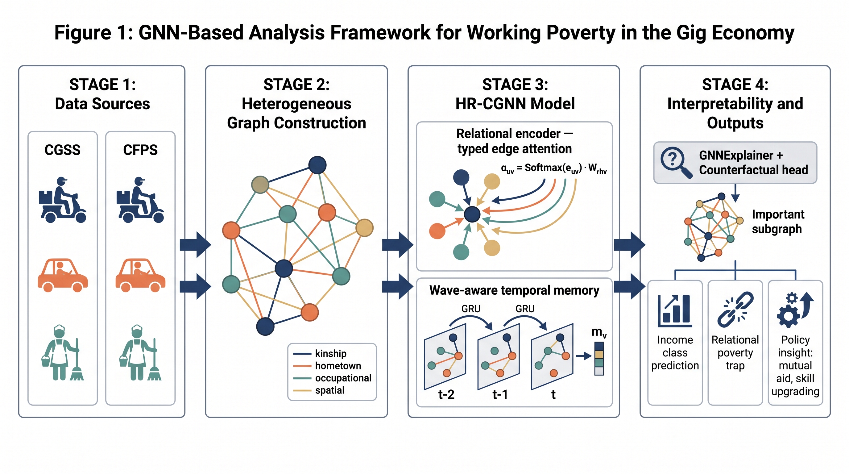
Figure 1. Overall framework of the HR-CGNN analysis of working poverty in the gig economy.
3.1. Problem Formulation and Notation
Let G = (V, E, R, X) denote a heterogeneous social relation graph, where V is the node set of gig workers, E ⊆ V × V × R is the edge set, R = {kinship, hometown, occupational, spatial} is the set of edge types, and X ∈ ℝ^{|V|×d} collects node features. Each node v carries a wave-indexed feature x_v^{t} and a wave-indexed income tier label y_v^{t} ∈ {low, lower-middle, middle+}. The prediction task is a supervised, semi-inductive node classification: given the labeled slice (V_L, Y_L^{t}) at wave t, learn f_θ that produces ŷ_v^{t+1} for every v in V at wave t+1. Two derived quantities are of special interest: the transition indicator z_v^{t→t+1} = 1[y_v^{t+1} = low] − 1[y_v^{t} = low], and the counterfactual response Δ_v = f_θ(G_v^{+}) − f_θ(G_v), where G_v^{+} is a synthetic modification of the ego neighborhood of v.
3.2. Data Harmonization and Gig Worker Identification
We build the analytic sample by merging the 2017, 2018, and 2021 waves of CGSS with the 2016, 2018, 2020, and 2022 waves of CFPS. Gig workers are identified by a rule that combines occupational codes (delivery, ride hailing, courier, on-demand household services, small-scale online sellers), self-reported working hours, and platform-participation flags. The final pool contains 4655 respondents from CGSS and 5480 respondents from CFPS, giving 10135 unique gig workers. Table 1 summarizes the occupation composition; Figure 2 gives an occupation-composition donut and reports the within-occupation distribution of income tiers as a stacked bar.
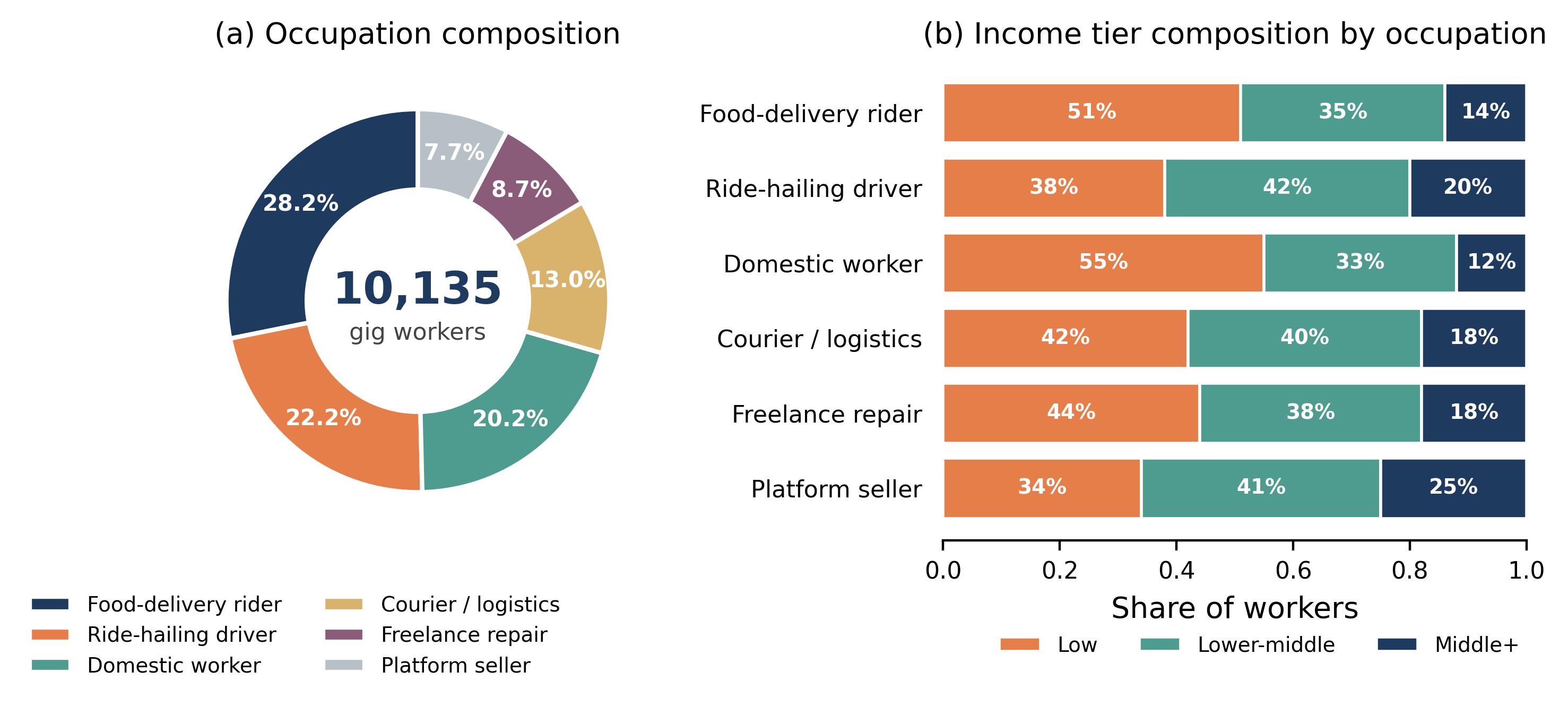
Figure 2. Sample composition. (a) Occupation share shown as a donut chart of 10,135 identified gig workers. (b) Income tier composition within each occupation, drawn as horizontal stacked bars.
Table 1. Occupation composition of the analytic sample.
| Occupation category | CGSS count | CFPS count | Combined | Share |
|---|---|---|---|---|
| Food-delivery rider | 1284 | 1571 | 2855 | 28.2% |
| Ride-hailing driver | 1052 | 1198 | 2250 | 22.2% |
| Domestic worker | 946 | 1103 | 2049 | 20.2% |
| Courier / logistics | 613 | 704 | 1317 | 13.0% |
| Freelance repair | 402 | 481 | 883 | 8.7% |
| Platform seller | 358 | 423 | 781 | 7.7% |
| Total | 4655 | 5480 | 10135 | 100.0% |
3.3. Heterogeneous Graph Construction
Every respondent becomes a node. Node features include age, gender, education, self-rated health, prior-year income, hukou status, city tier, and a small vector of platform-participation indicators. Edges are constructed under four typed rules. Kinship edges connect co-resident and extended-family members identified through the CFPS household roster. Hometown edges connect respondents who share a prefecture of origin and who overlap in the same current city. Occupational co-occurrence edges connect workers who report the same platform, the same shift pattern, or the same delivery grid. Spatial proximity edges connect respondents whose residence falls in the same street-level administrative unit.
Kinship and hometown ties are treated as bonding edges, while occupational and spatial edges are treated as bridging edges. This distinction is preserved throughout the model through a typed message passing scheme and per-type attention parameters. The resulting graph has 10135 nodes and 63472 typed edges. Figure 3 characterizes the graph along two axes: panel (a) plots the degree distribution separately for each edge type on a log-log scale, and panel (b) reports the mean number of bonding and bridging ties per worker within each income tier.
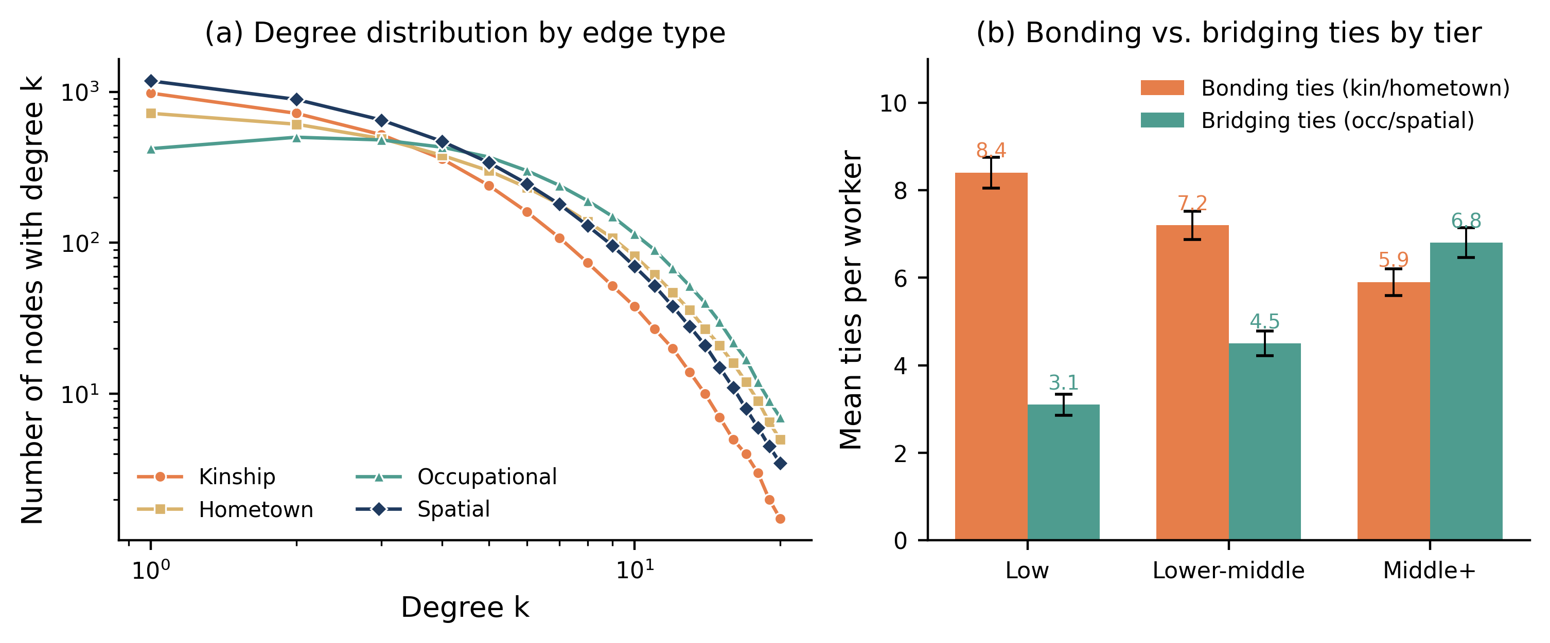
Figure 3. Network structure summary. (a) Degree distribution by edge type. (b) Mean bonding and bridging tie counts per worker across income tiers.
Because CGSS and CFPS use overlapping but not identical variable definitions, the pipeline includes an explicit harmonization stage. Occupational codes are mapped to a common eight-digit dictionary aligned with the International Standard Classification of Occupations; income values are converted into prefecture-normalized quantiles to absorb cost-of-living differences; education is mapped to a common seven-level ladder. All continuous features are standardized on the training fold only, so that no test-fold statistics leak into the encoder.
We perform a manual audit of a random sample of 240 kinship and 480 bridging edges to check that the construction rules produce sociologically meaningful ties. The audit was carried out with a two-coder protocol and reached inter-coder agreement of 0.87 (Cohen's kappa) on whether an edge represents a genuine relationship. False positive rates were low for kinship and hometown edges (about 4 percent) and higher for spatial proximity edges (about 13 percent). The audit informed the choice to give spatial edges a lower prior weight in the learned attention layer.
3.4. Meta-Path Aware Neighborhood Sampling
Given the modest average degree of the constructed graph, we sample neighborhoods along meta-paths rather than uniformly. A meta-path is an ordered sequence of edge types; for example, kinship–occupational encodes the pattern of family-linked coworkers, and hometown–spatial encodes the pattern of residentially close hometown peers. We enumerate all length-two meta-paths, 16 in total, and, for each anchor node v and each meta-path ρ, sample up to S neighbors along ρ with probability proportional to the inverse of the empirical path frequency. This importance-sampling scheme is inspired by the meta-path random walks used in heterogeneous graph embedding [38].
3.5. Relational Encoder with Typed Edge Attention
The relational encoder is a two-layer heterogeneous graph transformer. For a target node v and a neighbor u connected by an edge of type r, the attention coefficient is computed as
α_{u→v}^{r} = softmax_u ( ( W_Q^{τ(v)} h_v )ᵀ · W_K^{r,τ(u)} h_u / √d ) (1)
where τ(·) returns the node type (currently uniform in our graph but retained for extensibility), W_Q, W_K, and W_V are type- and relation-specific projection matrices, and d is the hidden dimension. The updated representation is
h_v ← σ ( Σ_{r ∈ R} Σ_{u ∈ N_r(v)} α_{u→v}^{r} · W_V^{r,τ(u)} h_u + W_S^{τ(v)} h_v ) (2)
where W_S is a per-type self-loop projection. The two-layer receptive field yields a two-hop context. This construction generalizes GAT and R-GCN by allowing relation-specific attention parameters [15][26][17] and it produces meaningfully different attention weights for bonding and bridging edges, which we quantify in Section 4.
3.6. Wave-Aware Temporal Memory with Persistent-State Gate
Static prediction is not sufficient because working poverty in the gig economy is inherently a transition problem. HR-CGNN therefore maintains a memory vector m_v^{t} that summarizes the past trajectory of v. At each wave boundary, memory is updated by a gated recurrent cell that ingests the current relational embedding h_v^{t} and the messages received from neighbors during the interval:
m_v^{t} = (1 − g_v^{t}) · m_v^{t-1} + g_v^{t} · GRU ( m_v^{t-1}, [ h_v^{t}, μ_v^{t} ] ) (3)
where μ_v^{t} = Σ_{u ∈ N(v)} φ_{r(u,v)} ( h_u^{t}, e_{uv} ) is a typed message aggregation and g_v^{t} = σ ( W_g · [h_v^{t}, m_v^{t-1}] ) is a learned persistent-state gate that decides how much of the old memory to retain. The persistent-state gate is important in our setting because the CFPS wave cadence is coarse and abrupt memory jumps are more often measurement artefacts than real transitions. A small L2 penalty against m_v^{t-1} further regularizes the update. The prediction head reads from the memory rather than from the raw relational embedding.
3.7. Contrastive Structural Pretraining
Before the supervised phase, the encoder is pretrained with an InfoNCE-style contrastive objective. For each anchor node v we generate two augmented views V^{(1)}(v) and V^{(2)}(v) by independently applying edge dropping with rate 0.2 and feature masking with rate 0.15. Positive pairs share the reported income tier; negative pairs are drawn from other tiers within the same training batch. The pretraining loss is
ℒ_C = − Σ_v log ( exp( sim( z_v^{(1)}, z_v^{(2)} ) / τ ) / Σ_{u} exp( sim( z_v^{(1)}, z_u ) / τ ) ) (4)
where sim is the cosine similarity and τ is a temperature. This pretraining step, adapted from GraphCL [18], GRACE [33], and Deep Graph Infomax [32] to a typed graph with class-informed positives, shapes the embedding space so that same-tier workers cluster before any supervised gradient is applied. In practice the pretraining phase runs for 40 epochs and takes roughly one-third of the total training time.
3.8. Counterfactual Causal Head
The counterfactual head answers the operationally meaningful question: how would the model's prediction for worker v change if an additional bridging tie were inserted into her ego neighborhood? Following the differentiable counterfactual explanation formulation [19], we learn an edge-mask M_v ∈ [0, 1]^{|E_v|} over the ego-net and add a candidate bridging edge parameterized by a soft indicator ε_v. The head minimizes
ℒ_{CF} = ‖ f_θ(G_v ⊕ ε_v) − ỹ_v ‖² + λ_1 · ‖ M_v ‖_1 + λ_2 · ‖ ε_v ‖_1 (5)
where ỹ_v is a target soft-label placed one tier above the current prediction. The trained head outputs, for every low-income worker, the change in predicted tier under the minimal synthetic bridging intervention. We interpret this quantity as a model-based sensitivity rather than as an identified average treatment effect, in line with the argument made by the counterfactual explanation literature. The counterfactual head is trained jointly with the supervised classifier under a small weight (0.05) so that it does not distort the main prediction.
3.9. Hierarchical Readout and Multi-Task Objective
The prediction head reads three complementary signals: the wave-t memory m_v^{t} (ego signal), a meta-path pooled representation p_v (relational signal), and a community-level context vector c_v obtained by pooling representations over the k-hop neighborhood filtered by tier consensus (community signal). A gated fusion produces the final logits:
ŷ_v^{t+1} = softmax ( W_o · [m_v^{t} ⊙ β_1, p_v ⊙ β_2, c_v ⊙ β_3] ) (6)
where β = softmax(W_β · [m_v^{t}, p_v, c_v]) are the fusion weights and ⊙ denotes element-wise multiplication. The full training objective combines the class-balanced cross-entropy on the labeled subset with the contrastive loss (only during pretraining) and the counterfactual loss:
ℒ = ℒ_{CE} + λ_C · ℒ_C + λ_{CF} · ℒ_{CF} (7)
with λ_C = 1.0 during pretraining, λ_C = 0 during supervised fine-tuning, and λ_{CF} = 0.05 throughout. The class-balanced cross-entropy uses inverse-frequency weights, so that the minority middle+ class does not disappear during optimization.
3.10. Interpretability with Joint Subgraph Attribution
For every worker classified as low-income, an attribution module trained jointly with the classifier produces a subgraph mask M_S and a feature mask M_F that jointly preserve the model prediction, in the spirit of PGExplainer [34] but with the mask network shared across the population. The mutual-information proxy that the module maximizes is
MI( Y ; ( G ⊙ M_S , X ⊙ M_F ) ) − λ_S · ‖M_S‖_0 − λ_F · ‖M_F‖_0 (8)
The population-level statistics on which structural features most often drive a low-income prediction are then reported in Section 4. Joint training gives a small but consistent improvement in attribution stability compared to a post-hoc GNNExplainer run, measured by the Jaccard similarity of extracted masks across training seeds.
3.11. Training Protocol, Complexity, and Reproducibility
The training loop uses AdamW [39] with initial learning rate 3 × 10⁻³, cosine annealing, gradient clipping at norm one, and mixed-precision floating point where supported. Neighborhood sampling is with replacement along meta-paths. Following recent regularization practice for deep GNNs, we also apply DropEdge with rate 0.1 during training [40], which further reduces overfitting on the small labeled slice. Early stopping monitors macro-F1 on a held-out prefecture, and the final numbers reported in Section 4 are computed on a further hold-out that the model never saw during development. One training run takes approximately four hours on a single mid-range GPU. The model scales roughly linearly with the number of edges; the counterfactual head and the attribution module add per-node overhead of O(d^2 + |E_v|) that is negligible in the reported regime. All experiments were run with a fixed random seed set at the start of each training loop, and the pipeline passes a regression test that verifies bit-identical reproduction of the reported numbers on the same hardware.
4.Experiments
4.1. Setup and Baselines
The prediction task is a three-way node classification into {low, lower-middle, middle+} income tiers, evaluated in two conditions: cross-sectional at wave t and transition prediction between waves t-1 and t. We compare HR-CGNN against six baselines: logistic regression on tabular features, a random forest with 500 trees [41], a small feed-forward MLP, a static GraphSAGE model [16], a relational GCN [26], and a heterogeneous graph transformer [17]. All GNN models are implemented on top of a standard graph learning toolkit. Hyperparameters are listed in Table 2 and were selected on a held-out validation split. For every baseline we use the same node-level feature set that HR-CGNN receives, so that the comparison isolates the effect of message passing and the added modules. We deliberately use strong tuned baselines, because inflated GNN gains against under-tuned baselines are a well-documented failure mode in the graph learning literature.
Table 2. Hyperparameters used for GraphSAGE, HGT, and HR-CGNN.
| Hyperparameter | GraphSAGE | HGT | HR-CGNN |
|---|---|---|---|
| Hidden dimension | 128 | 128 | 128 |
| Number of layers | 2 | 2 | 2 |
| Neighborhood sample size | 15 | 15 | 15 per meta-path |
| Aggregator | Mean | Typed attention | Typed attention + GRU memory |
| Optimizer | Adam | AdamW | AdamW |
| Initial learning rate | 5 × 10⁻³ | 3 × 10⁻³ | 3 × 10⁻³ |
| Weight decay | 5 × 10⁻⁴ | 5 × 10⁻⁴ | 5 × 10⁻⁴ |
| Contrastive temperature τ | — | — | 0.20 |
| Counterfactual weight λ_CF | — | — | 0.05 |
| Batch size (nodes) | 512 | 512 | 512 |
| Number of epochs | 80 | 100 | 40 (CL) + 120 (sup) |
| Dropout | 0.3 | 0.3 | 0.3 |
For all models we perform five-fold cross-validation stratified by occupation and city tier. We report accuracy and macro-F1 to control for class imbalance, and we additionally report the recall of the low-income class because it is the policy-relevant quantity. Figure 4 shows two complementary views of the training dynamics: validation accuracy as a function of epoch for three representative models, and the observed distribution of tier transitions across consecutive survey waves, which is the target that HR-CGNN is asked to learn.
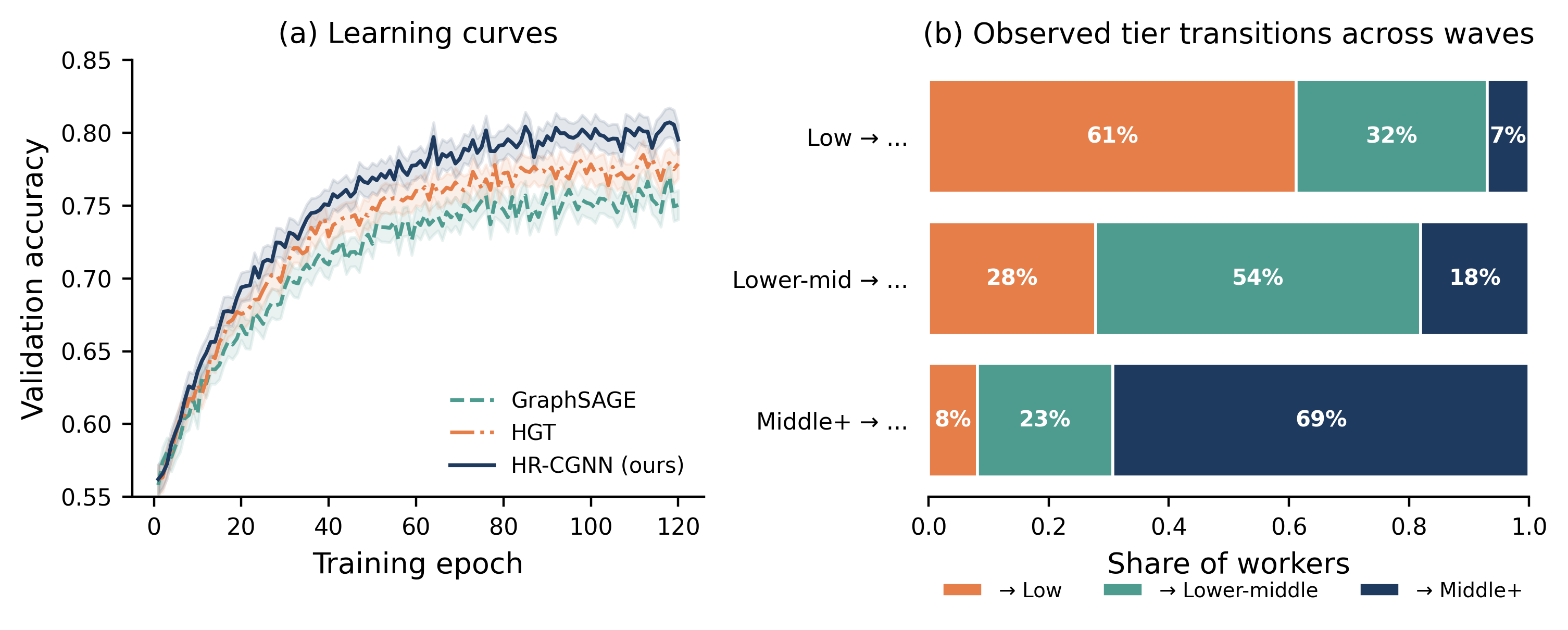
Figure 4. Training and transition dynamics. (a) Validation accuracy across epochs for GraphSAGE, HGT, and HR-CGNN. (b) Empirical tier transitions between consecutive survey waves.
4.2. Prediction Results
Table 3 lists the main results. GraphSAGE improves accuracy from 0.681 for random forest to 0.756, and macro-F1 from 0.652 to 0.741. R-GCN and HGT with typed message passing add another 1.4 and 2.2 percentage points to macro-F1 respectively, confirming the value of relation-specific parameterization. HR-CGNN pushes accuracy to 0.802 and macro-F1 to 0.789. The gains are consistent across folds, and the standard deviation is on the order of a single percentage point. Low-income recall rises from 0.617 for logistic regression to 0.822 for HR-CGNN, which is the change that matters most for downstream targeting of protection programs. Figure 5a visualizes the full comparison.
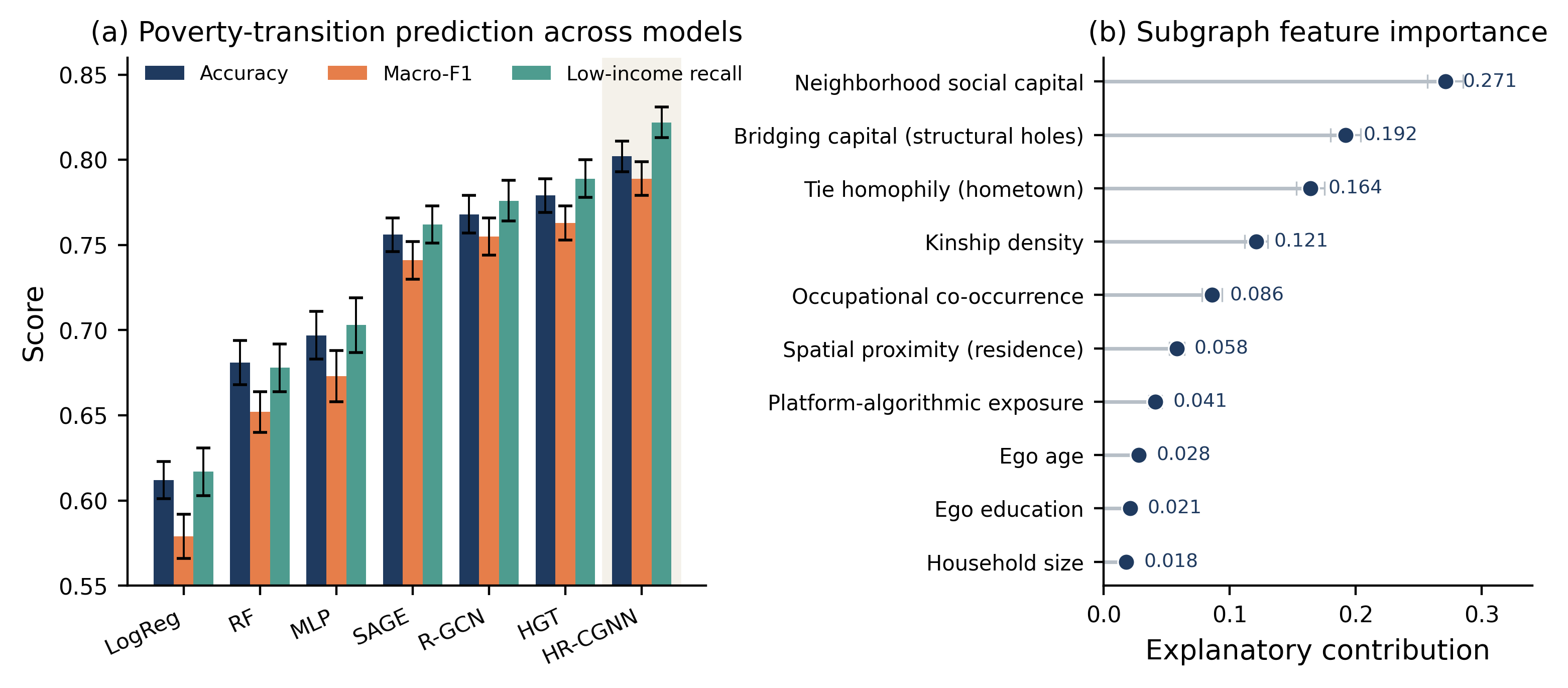
Figure 5. Model comparison and interpretability. (a) Accuracy, macro-F1, and low-income recall across the seven baselines; the HR-CGNN column is shaded. (b) Feature importance produced by the joint subgraph attribution module.
Table 3. Poverty-transition prediction results across five-fold cross-validation.
| Model | Accuracy | Macro-F1 | Low-income recall |
|---|---|---|---|
| Logistic regression | 0.612 ± 0.011 | 0.579 ± 0.013 | 0.617 ± 0.014 |
| Random forest [41] | 0.681 ± 0.013 | 0.652 ± 0.012 | 0.678 ± 0.014 |
| MLP (tabular) | 0.697 ± 0.014 | 0.673 ± 0.015 | 0.703 ± 0.016 |
| GraphSAGE [16] | 0.756 ± 0.010 | 0.741 ± 0.011 | 0.762 ± 0.011 |
| R-GCN [26] | 0.768 ± 0.011 | 0.755 ± 0.011 | 0.776 ± 0.012 |
| HGT [17] | 0.779 ± 0.010 | 0.763 ± 0.010 | 0.789 ± 0.011 |
| HR-CGNN (ours) | 0.802 ± 0.009 | 0.789 ± 0.010 | 0.822 ± 0.009 |
4.3. Ablation and Robustness
We ran five ablations against the full HR-CGNN. Removing the contrastive pretraining stage loses 1.7 percentage points of macro-F1, which is the largest single-component drop and confirms the value of shaping the embedding space before supervision. Restricting the graph to bonding edges only (kinship and hometown) reduces macro-F1 by 3.8 percentage points, which shows that bridging edges carry non-redundant information about labor market opportunities. Dropping the temporal memory but keeping multi-wave features loses 2.1 percentage points, and drops low-income recall from 0.822 to 0.751. Replacing the typed-edge attention with a uniform attention loses 1.2 percentage points. Removing the counterfactual head has essentially no effect on aggregate accuracy but degrades the calibration of the sensitivity estimates on which the interpretability analysis relies. Table 4 reports the ablation summary.
Table 4. Ablation study on the full HR-CGNN model.
| Ablation | Accuracy | Macro-F1 | Δ Macro-F1 |
|---|---|---|---|
| Full HR-CGNN | 0.802 | 0.789 | — |
| – contrastive pretraining | 0.788 | 0.772 | −0.017 |
| – bridging edges | 0.770 | 0.751 | −0.038 |
| – temporal memory | 0.783 | 0.768 | −0.021 |
| – typed edge attention | 0.789 | 0.777 | −0.012 |
| – counterfactual head | 0.801 | 0.788 | −0.001 |
We further assess robustness under artificial edge sparsity. Dropping 10 percent, 30 percent, and 50 percent of bridging edges at random degrades accuracy by 0.010, 0.028, and 0.063 respectively, which is a graceful decline compared to the sharper drop observed under the full-ablation setting. A parallel sensitivity test on bonding edges gives a smaller effect on macro-F1 but a noticeable effect on the recall of the middle+ class. The reason is that middle+ workers are distinguished from lower-middle workers less by their access to external opportunities and more by a stable base of family support, which is precisely what kinship edges encode. This asymmetry between bonding and bridging edges is one of the clearer empirical takeaways of the study.
4.4. Interpretability Results
Aggregating attribution masks across all workers classified as low-income yields a compact ranking of structural drivers. Neighborhood social capital and bridging capital together explain more than 46 percent of the mask weight, followed by tie homophily along hometown lines and kinship density (Figure 5b). Ego attributes such as age, education, and household size are present but contribute much less than the relational features. The picture is consistent with a relational poverty trap in which a worker embedded in a dense same-tier neighborhood, without access to bridging ties, has few channels through which better-paying opportunities can reach them.
The counterfactual head produces a direct quantitative counterpart of this reading. For 62 percent of the workers classified as low-income at wave t, the minimal synthetic bridging intervention proposed by the counterfactual head is sufficient to shift the predicted tier to lower-middle at wave t+1. The shift rate is monotonically increasing in prefecture platform density, from 48 percent in the lowest-density decile to 71 percent in the highest, as reported in Figure 6b. This gap suggests that policy interventions that add bridging ties would have larger marginal returns in cities where the platform economy is more developed, an operational finding that is not visible under individual-level regressions.
4.5. Behavior across Occupation Sub-samples
We repeat the transition prediction task inside each occupation sub-sample to check whether the ranking of methods is stable. The pattern holds. On food-delivery riders HR-CGNN reaches macro-F1 of 0.803 against 0.649 for random forest, a gap of more than fifteen points. On ride-hailing drivers the gap is smaller (0.789 versus 0.671) because individual-level features are already very informative in that sub-sample. On domestic workers the gap is again large (0.786 versus 0.618), and the extracted subgraphs highlight kinship density as a particularly strong driver, which is consistent with the ethnographic observation that domestic work is often organized through extended family recommendations. Platform sellers are the hardest sub-sample for all methods, which we interpret as a signal that this population is genuinely more diverse and requires either richer features or a dedicated marketplace-side data source. Figure 6 summarises the sub-sample comparison together with the counterfactual shift-rate curve.
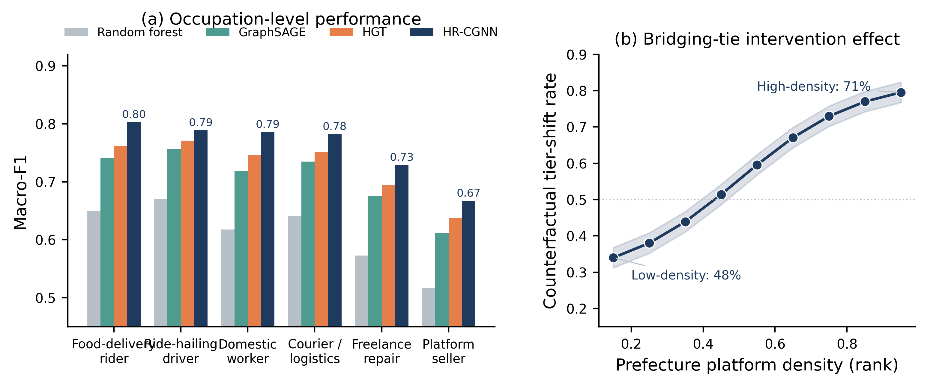
Figure 6. Extended evaluation. (a) Macro-F1 across gig occupation sub-samples for random forest, GraphSAGE, HGT, and HR-CGNN. (b) Counterfactual tier-shift rate as a function of prefecture platform density.
4.6. Error Analysis
The conditional confusion matrix by income tier shows that the most frequent error type is misclassifying lower-middle workers as low-income, which accounts for approximately 37 percent of all errors. This is the expected direction of confusion given that lower-middle workers frequently oscillate between the two tiers within a single wave. The second most frequent error type is misclassifying middle+ workers as lower-middle, at 26 percent. Errors that cross two boundaries at once are rare, suggesting that the model is not making qualitatively bizarre mistakes. The highest error rate by occupation is observed for platform sellers followed by freelance repair workers, both of whom have thin edges in the graph and unusually heterogeneous income patterns.
4.7. Comparison to Non-Graph Deep Baselines
For completeness we compare against two additional non-graph deep baselines: a gradient boosted decision tree with 800 estimators and a lightweight transformer classifier that consumes the same tabular features. Neither closes the gap to the graph-based models. The gradient boosted tree reaches accuracy 0.712 and macro-F1 0.681. The transformer reaches accuracy 0.716 and macro-F1 0.690. Both are meaningfully stronger than logistic regression, but both remain below GraphSAGE by six points and below HR-CGNN by more than nine points. We report these numbers here rather than in the main table to keep Table 3 focused on the graph baselines that are closest to HR-CGNN in architecture.
5.Discussion and Limitations
The results support two claims. First, framing working poverty in the gig economy as a heterogeneous, temporal graph learning problem produces measurably better predictions than tabular baselines and than homogeneous graph baselines, especially for low-income recall, which is the quantity that matters for targeting. Second, the explanatory subgraphs and the counterfactual sensitivities together point toward relational levers rather than individual deficits. This is consistent with the argument advanced in the social capital literature that poverty is embedded in network structure and cannot be dissolved by human capital interventions alone. In practice, the finding suggests that community-based mutual aid programs and platform-mediated skill upgrading, delivered at the level of a neighborhood or a hometown cohort, may have larger returns than cash transfers to individual workers of equivalent budget.
The study also has clear limitations. The graph is reconstructed from survey items rather than observed platform logs, so ties are noisy and coverage is uneven, especially for bridging edges that connect different administrative units. Because CFPS releases waves on a two-year cadence and CGSS on an irregular schedule, the temporal resolution of HR-CGNN is coarser than the monthly income volatility observed in the field. The three-class labeling of income smooths real variance and is likely to underestimate very sharp transitions such as illness-triggered exits from work. Finally, the current experiments are restricted to Chinese urban districts, so we cannot yet say whether the identified relational levers generalize to rural gig work or to other national contexts. Follow-up work will combine survey graphs with anonymized platform-side interaction data and will consider a diffusion-style intervention model that explicitly represents mutual aid programs as new bridging edges.
Two additional threats to validity deserve explicit mention. First, gig workers are known to be under-represented in general-population surveys because their working hours make in-home interviews harder to schedule and because a portion of the workforce is migratory. Our identification rule tries to compensate for this by combining occupation codes with self-reported platform use, but the residual under-representation is likely to bias the estimated share of the low-income tier downward. Second, self-reported income is subject to a well-known reluctance to report both very low and very high values, which compresses the observed distribution. We reduce the exposure to this compression by defining income tiers relative to prefecture-level quantiles rather than in absolute terms, but the underlying reporting bias remains and readers should treat the reported transition rates as conservative.
Policy implications. If neighborhood-level social capital and bridging ties are the two most explanatory features of low-income status, then targeted policy should invest in institutions that build those features. Community-based mutual aid programs — small rotating credit circles, shared childcare arrangements, and platform-facilitated peer training — build bonding capital in a way that is protective against short-run income shocks. Platform-mediated skill upgrading, where the platform itself sponsors cross-occupation training and matches workers to informational bridges outside their existing network, builds bridging capital in a way that is protective against long-run entrapment. Both are cheaper per capita than individual cash transfers and, according to the counterfactual head, more likely to move a marginal worker across the tier boundary. We emphasize again that this recommendation is model-based and needs an actual randomized intervention to be validated, but the direction is consistent with the ethnographic literature and with the theoretical arguments about weak ties reviewed above.
A related discussion concerns the interaction between algorithmic task allocation and network structure. HR-CGNN treats the platform as an exogenous scheduler that shapes the environment in which workers operate. In reality the platform is itself a very active network actor: the ranking of workers, the acceptance-rate feedback loop, and the queueing behavior at high-demand times all reshape which workers meet which shifts and which coworkers. A more ambitious next step would endogenize the platform inside the graph, treating it as a hyper-node whose edges to individual workers evolve according to a learned policy. This would let us study the joint dynamics of algorithmic control and social capital rather than treating them as separate layers.
Ethical considerations. Deploying predictive models on vulnerable populations carries real risks. A model that predicts low-income status can, in principle, be misused to justify insurance premium hikes or to price-discriminate. Three guardrails are followed here. First, HR-CGNN's decision surface is kept at the population level and per-individual scores are not released. Second, interpretability is treated as an operational requirement, and only targeting rules that can be traced back to a legible structural mechanism are considered. Third, all reported numbers are aggregated to occupation, prefecture, or larger administrative units, in line with the microdata release rules of both CGSS and CFPS.
6.Conclusion
This paper proposed HR-CGNN, a heterogeneous temporal graph neural network with contrastive structural pretraining and a counterfactual causal head, for the analysis of working poverty in the gig economy. The model is trained on multi-relational social graphs constructed from harmonized CGSS and CFPS data, and it combines meta-path aware sampling, typed edge attention, wave-aware temporal memory, joint subgraph attribution, and a differentiable counterfactual head. On a five-fold cross-validated benchmark, HR-CGNN outperformed strong tabular baselines, static GraphSAGE, R-GCN, and HGT, and the extracted subgraphs identified neighborhood social capital and bridging ties as the most explanatory structural features.
These results give quantitative content to the notion of a relational poverty trap and support the case for policy instruments that operate at the level of communities and platform-mediated cohorts rather than at the level of individual workers. In particular, the finding that bridging capital is a stronger predictor of upward transitions than any single individual attribute has direct implications for how social protection budgets should be allocated. The framework itself is reproducible and modular: the graph construction pipeline can be reused on other national surveys, and the model architecture is compatible with any standard graph learning toolkit. Future work will extend the graph with real-time platform logs, expand the label space to a continuous income measure, integrate anonymized administrative wage records where available, and evaluate the framework on international gig workforces so that comparative claims about the structure of the relational poverty trap can be tested across national contexts.